Chapter 8: Advanced Tools for Data Analysis
In the previous chapter you learned that by using simple tools like Google Sheets you can analyze thousands of rows of data to understand a bot’s activity. While Excel and Google Sheets can handle an impressive amount of data (more than 1 million rows and 16,000 columns for Excel and 400,000 cells for Google Sheets), these tools may not be suitable to run analyses on millions or billions of rows of complex data.
Every day, users create billions of posts, tweets, reactions, and other kinds of online data. Processing vast amounts of information like this is important for data sleuths who want to investigate human behavior on the web at a larger scale. In order to do that, you’ll need to familiarize yourself with programmatic analysis tools that can handle large data files. Even if you don’t end up using these tools on a regular basis, understanding each tool’s capabilities is vital when deciding which one to use.
In this chapter, we’ll practice reading in and exploring data using Python. During this process, you’ll be introduced to several more programming-related tools and concepts. You’ll learn how to set up a virtual environment, which is a contained, localized way of using libraries. After that, I’ll show you how to navigate the web application Jupyter Notebook, an interface you can use to write and modify code, output results, and render text and charts. Finally, you’ll install pandas, a Python library that enables you to do statistical analyses. As in the earlier chapters, you’ll absorb all this new knowledge through a practical exercise—ingesting and exploring Reddit submissions data.
Using Jupyter Notebook
In the previous chapters, we used Python through a command line interface and scripts. This was a great way for us to get acquainted with the coding language in a quick and straightforward way.
But as we build our Python skills and start working on more-complex scripts, we should look into tools to make these kinds of projects more manageable, structured, and shareable. The more complicated and longer our scripts become, the harder it is to keep track of every single step of our analysis.
This is where learning how to use Jupyter Notebook can be helpful. Jupyter is an open source web application that runs locally on your computer and is rendered in a browser like Chrome. Notebooks allow us to run our scripts in chunks, a few lines at a time, making it easier for us to adjust parts of our code as we iterate and improve upon it. The Jupyter Notebook web app, which evolved out of the web app IPython Notebooks, was created to accommodate three programming languages—Julia, Python, and R (Ju-Pyt-R)—but has since evolved to support many other coding languages.
Jupyter Notebook is also used by many data scientists in a diverse range of fields, including people crunching numbers to improve website performance, sociologists studying demographic information, and journalists searching for trends and anomalies in data obtained through Freedom of Information Act requests. One huge benefit of this is that many of these data scientists and researchers put their notebooks—often featuring detailed and annotated analyses—online on code-sharing platforms like GitHub, making it easier for beginning learners like you to replicate their studies.
Setting Up a Virtual Environment
In order to use Jupyter Notebook, you’ll need to take your coding skills to the next level by learning about three important concepts.
First, you’ll need to be able to create and understand virtual environments. Virtual environments can be challenging to wrap your head around, so let’s zoom out for a minute to examine their purpose.
As you’ve seen in the past few chapters, every time we’ve wanted to use coding libraries, we’ve had to install them by entering a command into a command line interface (CLI). Each library is installed in a default location on your computer, where it stays until it’s uninstalled.
For Python developers who are just beginning to use libraries and may need only one or two for their work, this approach may be sufficient. But as you become a more sophisticated researcher, you may require more and more libraries to handle different tasks. For example, some tasks may require a library capable of recognizing text from PDF image files, while others may call for a library that can take screenshots of a website. As you improve your skills and tackle more diverse projects, you may need to install more and more libraries in this default location, which runs the risk of causing conflicts between them. This is where virtual environments can be helpful.
A virtual environment allows you to install libraries only within a specified environment. Think of it like a parallel universe created for each project where you are allowed to experiment without affecting your overall computer’s environment. The virtual environment is like another computer inside of your computer. It enables you to take advantage of a coding library’s power without having to worry about how it interacts with other parts of your machine.
Although you can use various third-party tools for making virtual environments, for this project we’ll use Python 3’s built-in virtual environment tool. First, though, we need to make a python_scripts project folder to store our Jupyter notebooks. Once you’ve done that, open your CLI and navigate to that folder. As we saw in Chapter 3, the command to get inside a folder through the CLI is cd (which stands for “change directory”), followed by the folder’s path. If you stored your python_scripts folder in the Documents folder on a Mac, for instance, you would type this command into your CLI and hit enter:
cd Documents/python_scripts
For Windows, you would run this command:
cd Documents\python_script
Once you’re inside your folder, you can make a virtual environment by running this command if you’re a Mac user:
python3 -m venv myvenv
or this command for Windows users:
python -m venv myvenv
Let’s break down this command. First we tell our CLI that we’re using a command affiliated with python3 on Mac, or with python on PC. Then we use -m, a flag that tells Python 3 to call upon a module that is built into the programming language (flags allow you to access different functionalities that are installed onto your computer when you install Python). In this case we want to use the virtual environment module, venv. Last but not least, we give our virtual environment a name, which for simplicity’s sake we’ll call myvenv (you can call your environment anything you want, as long as the name has no spaces).
This command should create a folder inside your project folder with the name you gave it, which in this case is myvenv. This subfolder is where we’ll put all the coding libraries we want to install.
Okay, you’re almost ready to play in your virtual environment! Now that we’ve created this virtual environment, we start by activating it. Activation is like a light switch that turns your environment on and off using CLI commands.
If you’re still in the folder that contains your myvenv subfolder, you can simply enter this command to activate, or “switch on,” your environment (if not, navigate to the folder that contains your myvenv subfolder first). On Mac, this is the command:
source myvenv/bin/activate
On Windows, you would run this using the Command Prompt:
myvenv\Scripts\activate.bat
Let’s break down this code. The word source is a built-in command that allows us to run any source code contained in a path we specify (the source command can also be swapped out with a period, so the line . myvenv/bin/activate will do the same thing). In this case the path is myvenv/bin/activate, which tells the computer to go to the myvenv folder, then the bin folder inside myvenv, and finally the activate folder inside bin. The activate folder contains a script that switches your environment “on.”
Once you have run this code, your virtual environment should be activated! You can tell whether your environment is activated by looking at your command line: it should now start with the string (myvenv), parentheses included. To deactivate, or “switch off,” your environment, simply enter the command deactivate, and the string (myvenv) should disappear!
Welcome to a new level of programming. Now that you’ve learned how to create and switch your virtual environment on and off, we can start setting up Jupyter Notebook.
Organizing the Notebook
First let’s make sure we stay organized. While we’re not required to adhere to a specific folder structure, by organizing our input data, notebooks, and output data early on, we can help prevent errors in our analysis later. It’s also much easier to develop good habits early than to break bad ones later.
You need to create three separate folders that are stored outside of your myvenv folder but inside the overall project folder. First, you’ll need to create a folder called data to store input data, which consists of files you have received, downloaded, or scraped from APIs or websites and want to explore. Then you need an output folder, which will contain any spreadsheets you want to export based on your analyses. We won’t create spreadsheets in this book, but having an output folder is a great common practice for data analysts. The pandas library, which we will cover in “Working with Series and Data Frames” on page 143, offers a simple function called .to_csv() that allows for us to create .csv files from our analyses and that can easily be searched for on Google. Finally, we’ll keep our Jupyter notebooks in one neat folder called notebooks.
You could create these folders, or directories, manually on your computer, but you can also create them programmatically using the mkdir command. To do this, navigate to your overall project folder in your CLI (if you’re still in your myvenv folder, move up using cd ..) and enter these three lines:
mkdir data
mkdir output
mkdir notebooks
The command mkdir makes a directory with the name you specify. In this case, the three commands create the three folders just described.
Alternatively, you can use the mkdir command followed by all three folder names separated by a space, like so:
mkdir data output notebooks
Installing Jupyter and Creating Your First Notebook
Jupyter allows us to create notebook documents that can read different kinds of code, such as Python and Markdown, a language often used to format documentation. Because it is able to read various coding languages, a notebook can render the results of Python code alongside formatted text, making it easier for programmers to annotate their analyses.
What’s even better is that we can download Jupyter Notebook from the web and install it on our computers like any other Python library: via pip. To install Jupyter Notebook, open your CLI and enter the following command:
pip install jupyter
Now you can launch it by running the following command from your project folder:
jupyter notebook
When you enter this command in your CLI, Jupyter Notebook will launch a local server, which is a server that runs only on your computer, and open a window in your default web browser, which, for the purposes of this book, should be Chrome.
You can see the Jupyter Notebook interface in Figure 8-1.
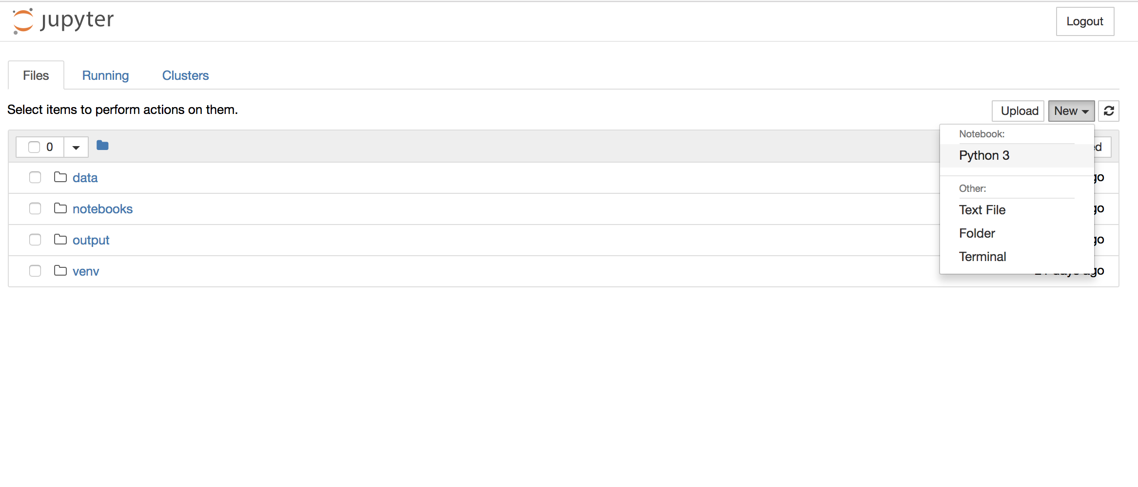
Figure 8-1: The Jupyter interface
This interface allows us to navigate into folders and create files in them. For this exercise, navigate into the notebooks folder and then, from the drop-down menu, select New>Python3. This should create a new notebook inside the notebooks folder and open it in a new tab.
Jupyter notebooks look a lot like your average text document software, with editing tools and a full menu of options, except that they are, of course, tailored to the needs of a Python developer. What’s particularly nifty about them is that they use cells to run different chunks of Python code one at a time. In other words, you can separate out your Python code into multiple cells and run them one by one.
Working with Cells
Let’s give it a whirl. Your notebook creates a cell by default, which has the text In [ ]: and a text field where you can enter code. In that cell, enter this line of Python code:
print(“Hi”)
Select the cell containing this code and press the Run button (or use the shortcut shift-enter). This should execute the Python code that you just typed in the cell. In this case, the notebook should print the results of your code directly below the cell and create a second cell, as shown in Figure 8-2.
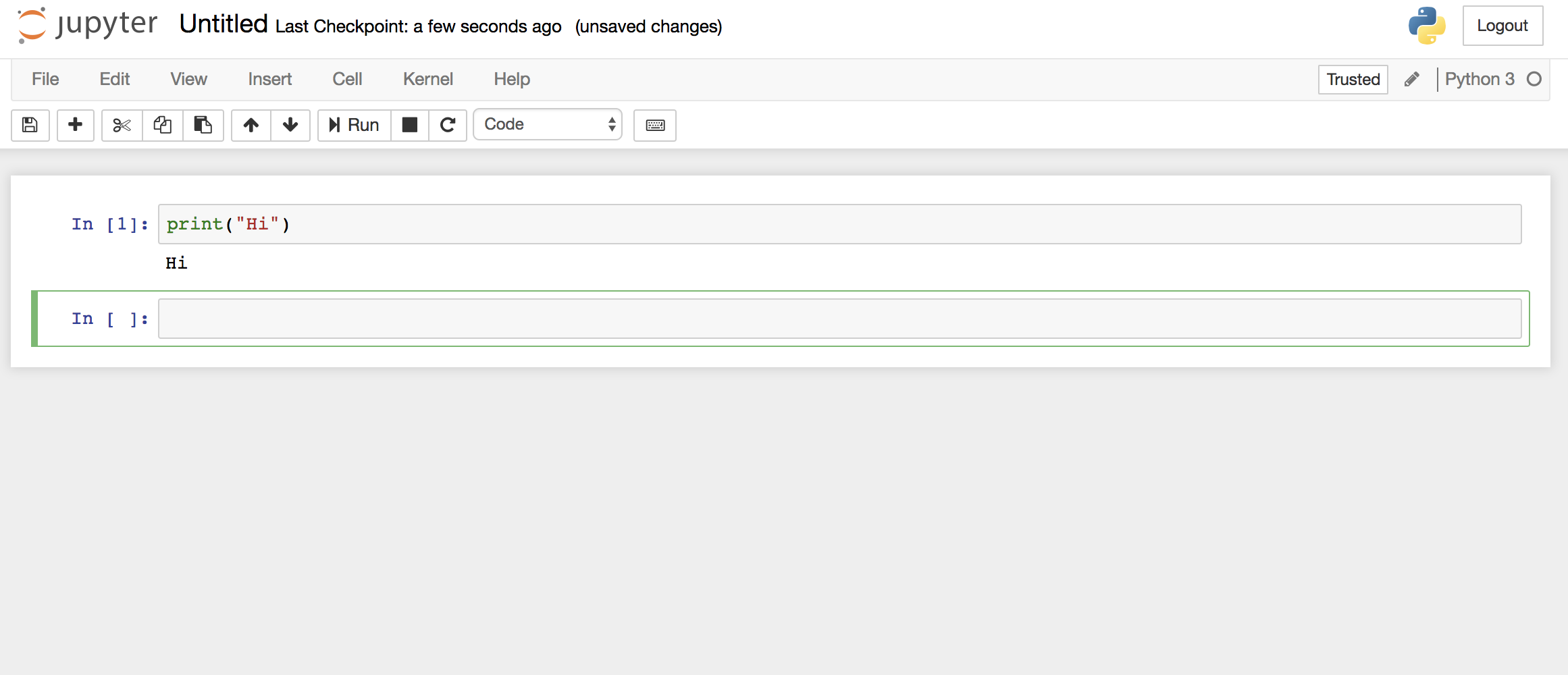
Figure 8-2: Two cells inside a Jupyter notebook
Congratulations! You have written your first notebook and run your first cell of Python!
There’s one important thing to note here: now that Jupyter has run your cell, the square brackets to the left of the cell should no longer be empty. Since this is the first cell we ran in this notebook, they should contain the number 1.
What happens when we run the same cell with different code? Let’s find out. Delete the code inside the first cell and enter the following code:
print("Hello!")
Now select the cell by clicking the area to the left of it (a blue bar should highlight the left side of whichever cell you’re currently selecting). Then click the Run button again.
The cell should render the string Hello!, just as it did the string Hi before. But now the square brackets should contain the number 2. As you can see, Jupyter Notebook tracks not only the fact that you’ve run a cell but also the sequence in which you run it.
This kind of tracking is very important since the code in your notebook is separated into cells. Unlike a script, which runs top to bottom in one sitting, cells can be run out of order and one at a time. Tracking tells you exactly what code your notebook has already run and which code it still needs to run. This can help you avoid common Jupyter errors, like when code in one cell refers to a variable defined in a cell you haven’t run yet.
Similar to text-editing software like Microsoft Word or TextEdit, Jupyter Notebook comes with a number of great tools in a visual interface. You can use the toolbar to do things like save your notebook (the floppy disk icon), cut cells (scissors icon), add cells (plus sign), and move cells up (up arrow) or down (down arrow).
Now you know the basics of how to run cells of Python code in Jupyter Notebook. But as you experiment more with code by rewriting, rerunning, deleting, or moving cells to improve your notebook, you might find you’re storing a lot of “garbage” in the notebook’s memory. For example, you might create variables you eventually decide to delete or store data that you later realize you won’t use. This garbage can slow your notebook down. So how can you clear the memory of any Python code you’ve run in a notebook without destroying the lines of code you’ve written inside your cells?
There’s a lovely trick for that: go to the menu and select Kernel> Restart, which will clear all previously run code and any numbers within the square brackets next to the cells. If you run a cell again, it should render the results of your code and fill the square brackets with the number 1.
Last but not least, there’s a great option for running multiple cells in a sequence. To illustrate it, let’s first add another cell to our notebook. Click the plus sign (+) button, and then enter this code in the second cell:
print("Is it me you're looking for?")
While we’re at it, why not add two more cells? One cell contains this code:
print("'Cause I wonder where you are")
and the other contains this line of code:
print("And I wonder what you do")
To run all four of these cells in sequence, select the first cell, which contains the line print(“Hello!”). Then select the menu option Cell> Run All Below. This should automatically run all the cells, starting with the one we selected and going all the way to the bottom. (Or, if one cell contains an error, our notebook will stop there!)
Notebooks can be used for a variety of tasks, and these rudimentary steps should get you started exploring Jupyter Notebook as a tool for data analysis. You can run almost any code you have written in a script as a notebook. You can even take the previous scripts you’ve written for this book, split the code up into cells, and run the code one chunk at a time.
Now that you’ve seen how to use the Jupyter Notebook interface, let’s turn to exploring Reddit data with pandas.
What Is pandas?
Throughout this book, you’ve learned how to use various libraries to help you gather data. Now it’s time to learn about a library that will help you analyze data.
Enter pandas.
Despite what you might guess, the pandas library has nothing to do with the adorable, bumbling bears native to Asia. The library actually got its name from the concept of panel data—a data set that spans measurements over time—and was constructed by its creator, Wes McKinney, to handle large, longitudinal data sets. It allows Python to ingest data from a variety of sources (including .csv, .tsv, .json, and even Excel files), create data sets from scratch, and merge data sets with ease.
To use pandas, as with Jupyter and other libraries, we first have to install it using pip. If you’ve followed all instructions thus far and have turned on your notebooks, you’re also running a local server through your CLI that powers Jupyter Notebook. One way to tell if your local server is currently running Jupyter Notebook is to look for brackets containing the letter I, a timestamp, and the word NotebookApp, like this: [I 08:58:24.417 NotebookApp]. To install pandas without interrupting that local server, you can open a new window in your Terminal (leave the one running your server open!) or your Command Prompt, navigate to the same project folder, turn on your virtual environment again, and then install the new library.
Once you have followed those steps, you can execute this pip command to install pandas:
pip install pandas
After installing the library, you need to import it. The most conventional way to do so in a Jupyter notebook is by typing an import command into a cell and running it:
import pandas as pd
In this example import command, we’ve imported pandas and will be able to access its functions using the shorthand pd. In other words, when you use this command, instead of referring to the library as pandas throughout your code, you would call pd. So, for example, you would write pd.Series([12,53,57]) instead of pandas.Series([12,53,57]). This import command is a convention used by many data analysts who work with pandas and helps keep code neat and easy to read.
Now let’s start creating, reading, and manipulating some data structures!
Working with Series and Data Frames
One of the simplest data structures that we can load into pandas is a series, which is similar to a list or an array. To make a series in pandas, we can use the Series() function.
In a new cell below the one containing the import pandas as pd line, enter these two lines:
① numbers = [12, 53, 57]

② pd.Series(numbers)
The code stores the list of numbers [12, 53, 57] in the numbers variable ①. In the next line, we call up the pandas library by its shorthand, pd, followed by a period and then the Series() function, to which we pass the argument numbers ②. In other words, we’re using the Series() function to make a data object of the type series, and placing the list of numbers into this series. This is the same way we accessed the functions within another library, Beautiful Soup, in Chapter 4: we first refer to the library via the shorthand that we assigned to it, and then we access the functions that it offers through their names.
Once we run that cell, the notebook should display the following text right under it:
0    12
1    53
2    57

dtype: int64
This is how pandas represents a simple data series, which can also be referred to as a one-dimensional data set. On the left side, there’s a column that represents the index, or the position, of each data item. The index starts with 0, as is customary, and increments by 1 with each row. On the right side are the actual data values. At the end of the series you’ll see the words dtype (data type) and int64 (integer), separated by a colon.
Note Similar to dtype and int64, strings are denoted by object and floats by float64. There are other data types, too, including datetime64, which stands for date and time values, but we won’t need them for now.
A series is perhaps the simplest kind of data set: it’s one column of data where each row contains a value. But in pandas you are more likely to use a two-dimensional object that’s able to handle multiple columns: a data frame. Think of a data frame as a spreadsheet that is read by Python instead of being opened in Excel or Google Sheets, and can hold a lot more data. Not unlike a spreadsheet, a data frame has an index (row labels) and columns (column labels).
To make a data frame, you can use pandas’ built-in DataFrame() function. Let’s give it a try. In a new cell, enter the following dictionary and line of code:
① numbers2 = {"one": [1.2, 2, 3, 4],

              "two": [4, 3, 2.5, 1]}

pd.DataFrame(numbers2)
As before, we’re creating a variable to store our data: numbers2 ①. Then we assign the variable numbers2 a dictionary, where the key “one” is assigned the list of values [1.2, 2, 3, 4] and the key “two” is assigned the list of values [4, 3, 2.5, 1]. We’re adding a line break between those two dictionary items within the braces for legibility, but it will not interfere with running your code.
You can see how Jupyter renders this code in Figure 8-3.
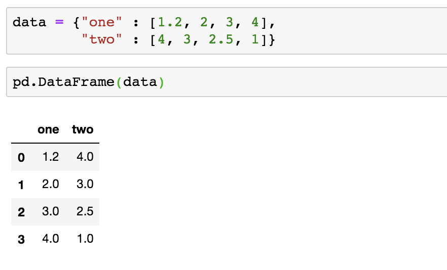
Figure 8-3: Two cells and a data frame rendered as a table
Like a series, this data frame features an index, which appears as a column on the leftmost side. The data frame also has two columns, named one and two, that contain our numerical data.
Reading and Exploring Large Data Files
Data sets come in all sizes and levels of detail—some are fairly straightforward to understand while others can be quite convoluted, large, and unwieldy. Social media data can be especially difficult to manage: online users produce a large amount of data and content that, in turn, can produce many reactions, comments, and other responses.
This complexity can be compounded when we’re dealing with raw data from a social media company, academics, or other data archivists. Often, researchers will collect more data than they need for individual analyses because it’s easier to ask various questions of one large data set than to have to collect smaller data sets over and over again for projects that may change in objective and scope.
Due to API restrictions, it can be difficult for researchers, journalists, and other analysts to track media manipulation campaigns, trolling attacks, or other short-term online phenomena. To name one example, by the time Congress released the Twitter handles and names of Facebook pages that Russian operatives used to manipulate the 2016 US election, the accounts had been erased and were no longer traceable by researchers for examination.
As a countermeasure, various institutions and individuals have started harvesting and storing this social media data. The Internet Archive, for instance, does a monthly data pull and hosts millions of tweets on its servers that researchers may use for linguistic or other analyses. Academics have collected and archived Facebook information in an attempt to better understand phenomena like the spread of hatred against Muslims in Myanmar.
While these efforts are immensely helpful for doing empirical research, the data they produce can present challenges for data sleuths like us. Often we have to spend a considerable amount of time researching, exploring, and “getting to know” the data before we can run meaningful analyses on it.
Over the next few pages, you’ll learn how to read and explore one such large data file. In this chapter and the coming ones, we’ll look at Reddit data made available by Jason Baumgartner, a data archivist who believes it’s vital to make social media data available to scholars and other kinds of researchers. This data contains all submissions between 2014 and 2017 made to r/askscience, a Reddit forum, or “subreddit,” where people ask science-related questions. For the rest of this chapter, we’ll get to know the data set’s structure and size through pandas. You can download the data set here: https://archive.org/details/askscience_submissions/.
Once you’ve downloaded the data, you need to place it into the correct folder. In this case, that’s the data folder you created earlier.
Then you need to go to the Jupyter notebook you created. The first cell, as is convention, should still contain the import pandas as pd command, since all import statements should run first. In a cell after that, load the .csv spreadsheet in the data folder as follows:
reddit_data = pd.read_csv("../data/askscience_submissions.csv")
The name reddit_data refers to the variable we create to store the Reddit data we’re ingesting. Then, using the equal sign (=), we assign this variable a data frame that we create using the pandas function read_csv(). The read_csv() function requires as an argument the path to a data file (this is usually a .csv file, but read_csv() can also handle .tsv and .txt files as long as they contain data values that are separated by a comma, tab, or other consistent delimiter), and this argument needs to be a string. Since we’re running the command inside a notebook, the path needs to reflect where the data file is located in relation to the notebook file. Using the two dots and forward slash allows us to navigate to a folder one level above our current folder (notebooks), which in this case is our project folder (python_scripts). Then we navigate into the data folder, which contains the .csv file named askscience_subsmissions.csv that you placed in the folder earlier.
Note The data is over 300MB and may take several seconds to load. Loading it on my computer took a good 10 seconds.
Once we run that cell, pandas will create a data frame that is stored inside the variable reddit_data.
Looking at the Data
Unlike programs like Excel or Sheets, which are constructed for users to manipulate data through visual interfaces, pandas will not actually render an entire data frame at once. You may have noticed that just now, pandas didn’t render the data at all. This is because you assigned the output of read_csv() to a variable, storing rather than returning or printing it. If you run the function without assigning it, or run a cell with the reddit_data variable in it, you’ll see a snippet of the data. While this truncation can be disorienting at first, it also saves a lot of computing power. Some software can crash or slow down when you open files containing a few hundred thousand rows, depending on their complexity. Thus, by not displaying the full data frame, pandas allows us to work more efficiently with much larger data sets.
This means that we need to find a way to read the different parts of our data set. Thanks to the pandas developers, we can do this very easily with a few handy functions.
To look at the first few rows of our data set, we can use a function called head(). This function takes an integer as its only argument, and defaults to 5 if you enter nothing. So if you want to see the first 10 rows of your data set, you could run a cell with this line:
reddit_data.head(10)
In this command, first we call upon the reddit_data variable that holds the data we ingested through the .csv file. Then, we call the head() function on the data in the variable. Jupyter Notebook should render the data frame as shown in Figure 8-4.
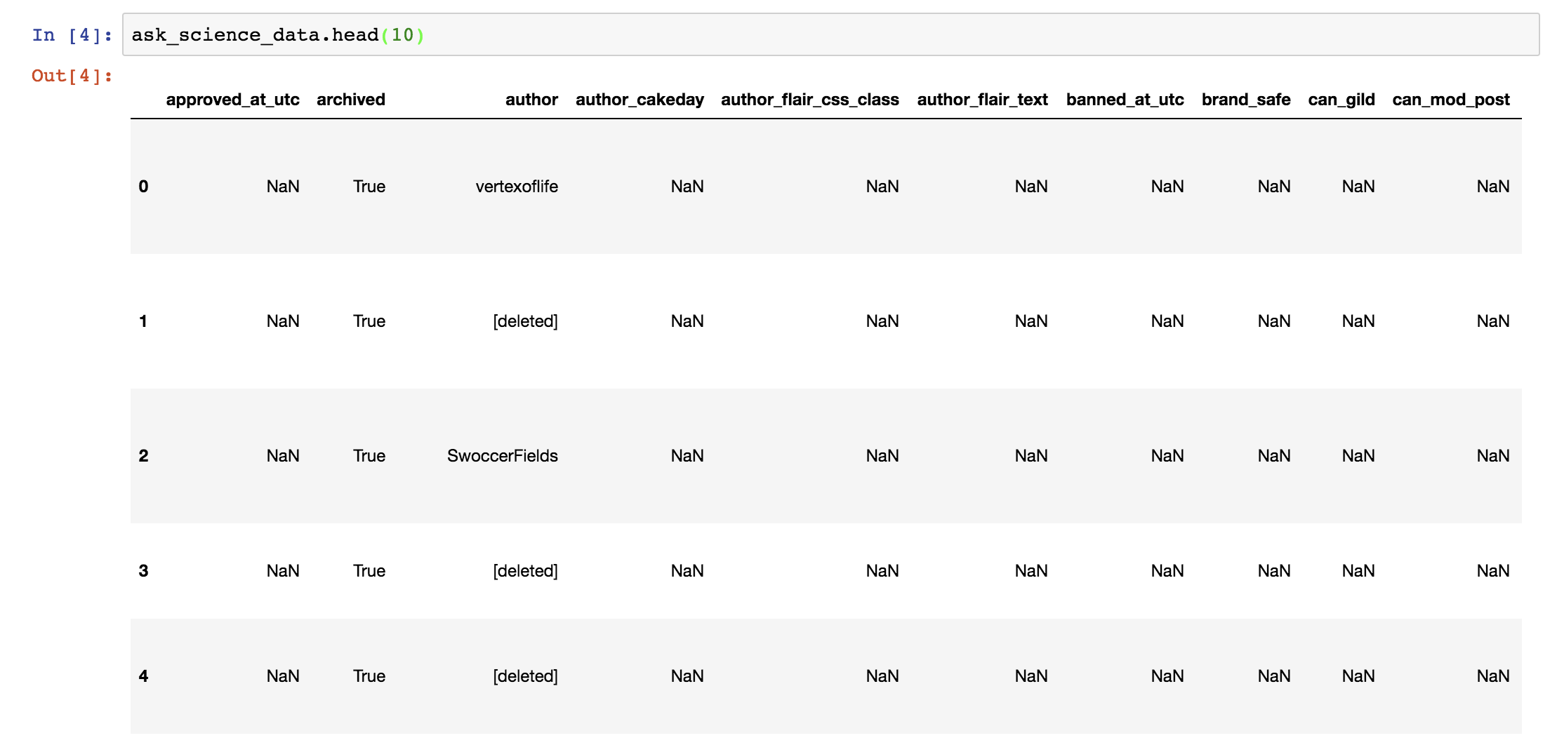
Figure 8-4: Rendering the first 10 rows of the data frame
To see the last 10 rows of a data frame, you can use the tail() function, which follows the same structure:
reddit_data.tail(10)
Once you run your cell containing this code, you’ll see the same rendering of your data frame as you did with the head() function, except for the last 10 rows of your data frame.
While you can’t see the entire data set at once, that may not be all that important for now. Remember you’re getting to know your data set right now. That means you want to know what kind of values each column contains and what the column names are. Seeing the first or last 10 rows of your data can certainly help with that.
You may have noticed, however, that you have to scroll sideways to reveal every single column of your data set. That can be a little unwieldy. Fortunately, there are some built-in tools that you can use to help summarize parts of your data set.
You can transpose your data set to see the column headers as rows and your data as columns. Transposing allows us to basically flip the data frame—it will look a bit like we just rotated the table 90 degrees counterclockwise. To do this, you append your call to the data set with a T like this:
reddit_data.T
To see all the column names as a list, you can use this line of code:
reddit_data.columns
To get a summary of all the data types that your data frame contains, use dtypes:
reddit_data.dtypes
Finally, you can use good old vanilla Python to find out the number of rows in your data frame. Remember the print() function we used back in Chapter 1 to display information in the interactive shell? We used it to find the length of a string or the number of items in a list using len(). We can also use these functions to see how large our data frame is:
print(len(reddit_data))
This code might look more complicated than it really is. First we use the len() function to measure the length of the data frame (that is, the number of rows it contains) by passing it the argument reddit_data, which is our data set. In other words, first we get the length of the reddit_data data frame. When used by itself, the len() function renders results only if no other statements follow it inside a cell, so it’s good practice to place it inside a print() function to make sure the cell renders the result of what len() measured.
The number you should get is 618576 (or, more legibly to humans, 618,576). That represents the number of rows in our data frame.
If we run the same set of functions and pass reddit_data.columns as an argument to len(), we can get the number of columns in the data frame:
print(len(reddit_data.columns))
This line measures the length of the list of columns within the data frame. This particular data frame contains 65 different columns. So, if you multiply 65 columns of data by 618,576 rows, you find that we’re dealing with more than 40 million values. Welcome to the big data leagues!
Viewing Specific Columns and Rows
Now we know how to get a feel for the structure of our data frames, meaning we know how to get a bird’s-eye view of our data. But what if we want to take a closer look at specific parts of our data? That’s where square brackets come in.
When tacked onto the variable that contains our data frame, square brackets can allow us to select, or index, different subsets of data. For instance, to view a specific column, you can specify the column’s name inside the brackets as a string. In this line, we’re selecting the column named title:
reddit_data["title"]
This lets us focus on just the column containing the values that are categorized as the title of each Reddit post. Fun fact: when run on its own, this line of code will render the column, but you can also use it to store a copy of a data column in a variable, like this:
all_titles = reddit_data["title"]
We can also view multiple columns with bracket notation, by assigning a list of them to another variable:
column_names  = ["author", "title", "ups"]
reddit_data[column_names]
First we create a variable called column_names to store a list of column names as strings. Keep in mind that each column name must be the exact string in the data set itself, capitalization included. Then we place this list inside the brackets to display just those columns.
There are also nifty ways to isolate individual rows. As we saw earlier in this chapter, each row has an index, which acts kind of like a label. By default, pandas assigns each row an integer as an index (we can assign each row custom indexes, too, but we won’t do that in this exercise). We can use the iloc[] method to call on any given row by placing the row’s index number inside the brackets (in programming lingo, this is referred to as integer-location-based indexing):
reddit_data.iloc[4]
If we run a cell with this line, we should see the fifth row of the data set (remember that programming often starts counting from 0).
Last but not least, we can combine these two methods. If, for instance, we want to call up the column named title and display only the value in the fifth row, we can do that like so:
reddit_data["title"].iloc[4]
These are just a few ways in which we can get to know our data set better. And this is no small feat, given that we’re dealing with millions of values contained in what is essentially one large spreadsheet.
Now that you have all the basics down, you can start learning how to do calculations with the data.
Summary
You’ve now seen how to explore large data sets, which is an important first step for any data analysis. Only after we understand the nature of the data—its contents, formats, and structure—can we find the best strategies to analyze it for meaning.
In the next chapter, we’ll continue working on this Jupyter notebook and discover ways of asking questions of our data set.