Chapter 10: Measuring the Twitter Activity of Political Actors
In Chapter 9, we did our first data analysis with a large data set and saw how we could answer a research question based on a simple categorization. Although it produced good results, that sort of analysis is limited: it looked at the data at only one point in time. Analyzing data across time, on the other hand, allows us to look for trends and better understand the anomalies we encounter. By exploring the changes in data and isolating specific events, we can make meaningful connections between them.
In this chapter, we’ll look at data as it changes over time. Specifically, we’ll examine a data set Twitter published in 2018 that consists of tweets political actors based in Iran posted before, during, and after the 2016 US presidential election to influence public opinion in the US and elsewhere. The data dump is part of the platform’s ongoing efforts to allow researchers to analyze media manipulation campaigns run by false and hired Twitter accounts. We want to look at tweets that used hashtags relating to Donald Trump and/or Hillary Clinton and determine how they behaved over time. Did they increase in the lead-up to the election? Did they drop right after the 2016 election or continue to grow?
Along the way, you’ll learn how to filter data using a type of function called a lambda. You’ll see how to format raw data and turn it into a time series or resample it. Last but not least, you’ll learn about a new library to use alongside pandas, called matplotlib (https://matplotlib.org/). The matplotlib library will help us make sense of our data by visualizing it within the Jupyter Notebook environment, using simple graphics to illustrate data fluctuations. By the end of this project, you should have a strong grasp of pandas and the kinds of things you can do with it.
Getting Started
In 2017 and 2018, Twitter, Facebook, and Google were heavily criticized for allowing international agents to spread false or misleading content meant to influence public opinion in the US and abroad. This public scrutiny ultimately led to the publication of two major data bundles: one of Russian tweets that—according to Twitter, Congress, and various media reports—were used to manipulate the US media landscape, and another of Iranian tweets doing the same.
The Russian data set is much larger and could slow down our progress, as it would take a long time for it to load and process. So, as mentioned earlier, we’ll focus on the other data set: the Iranian data. In particular, we’ll be looking at the spreadsheet titled iranian_tweets_csv_hashed.csv, which you can download directly from https://archive.org/details/iranian_tweets_csv_hashed/.
Our research question is straightforward: How many tweets related to Trump and Clinton were tweeted by Iranian actors over time? We’ll define Trump- and Clinton-related tweets as tweets that use hashtags containing the string trump or clinton (ignoring case). As discussed in Chapter 9, this kind of categorization may miss some tweets related to the two presidential candidates, but we’re only doing a simple version of this program for teaching purposes. In a real data analysis, we’d likely cast a wider net.
Now that we have a research question, let’s get started on the project!
Setting Up Your Environment
As we did in the previous chapter, first we’ll need to set up a new folder for our project. Then, within that folder, we’ll need to create three subfolders: data, notebooks, and output. Once you’ve done that, place the downloaded Twitter data in the data folder.
Next, navigate to your project directory inside your CLI and enter python3 -m venv myvenv. This creates a virtual environment inside your project, which you can activate using the command source myvenv/bin/activate. Your virtual environment is activated if your CLI begins with (env) (revisit Chapter 8 if you need a refresher).
With the virtual environment activated, now we need to install all the libraries we’ll be using. We want jupyter, pandas, and matplotlib, all of which we can install using pip as follows:
pip install jupyter
pip install pandas
pip install matplotlib
After installing all three libraries, enter jupyter notebook into your console and, once Jupyter starts, navigate into the notebooks folder and create a new notebook by selecting New>Python 3. Lastly, let’s rename the new notebook: click the title, which usually defaults to Untitled, and rename it twitter_analysis.
With all that done, you’re ready to go!
Loading the Data into Your Notebook
First, let’s ensure that we can use all the libraries we’ve just installed. To load pandas and matplotlib, we’ll use the import statement. In the first cell of your notebook, type the following:
import pandas as pd
import matplotlib.pyplot as plt
In the first line, we’re importing pandas and using pd as shorthand so we can simply refer to pd to access all of the library’s functionalities. We’ll do the same in the second line for matplotlib, except here we only need a subset of functions called pyplot, which we’ll call plt as a shortcut. This means, instead of having to write out matplotlib.pyplot, we can simply use plt, which should help avoid cluttered code.
Note The convention of using pd as shorthand appears in the documentation for the pandas library. Similarly, the plt shortcut is used in the matplotlib documentation.
Click Run (or use shift-enter) to run this cell, and you should be able to access both libraries in the cells that follow.
Next, we need to load in the data. Let’s create a variable called tweets to hold the data we want to examine. Enter the following into the next cell and run it:
tweets = pd.read_csv("../data/iranian_tweets_csv_hashed.csv")
This line ingests the Twitter data in our data folder using the pandas function read_csv(), which takes a filepath to a .csv file and returns a data frame we can use. For a refresher on data frames, check out Chapter 8.
Now that our data is ingested, let’s think about the next step we need to take. This data set includes tweets covering a wide array of topics, but we’re interested only in tweets about Donald Trump and Hillary Clinton. This means we’ll need to filter our data to only those tweets, just as we did in Chapter 9 when we filtered our r/askscience data to posts relating to vaccinations.
Once again, before we can narrow it down, we need to get to know our data a little better. Since we’ve already loaded it, we can begin exploring it using the head() function. Enter the following into a cell and run it:
tweets.head()
You should see the first five rows of data, as shown in Figure 10-1.
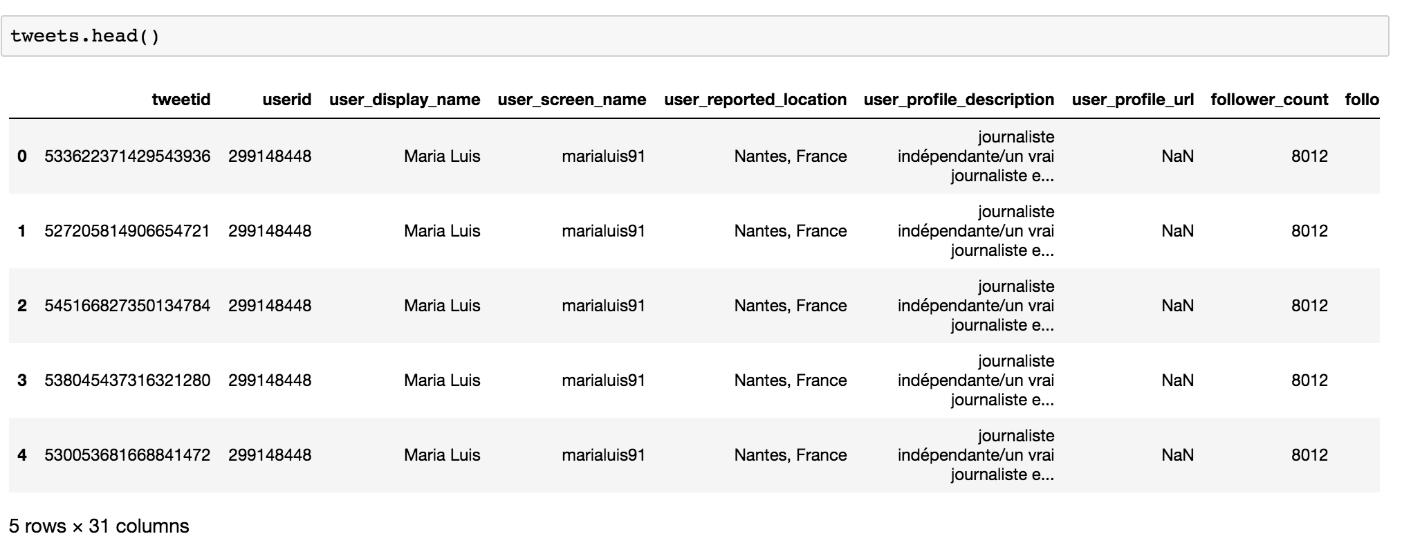
Figure 10-1: The loaded data frame
As you can see, this dump contains a large assortment of metadata related to the tweets. Every row represents one tweet and includes information about the tweet itself as well as the user who tweeted it. As you might remember from Chapter 8, to see all the column names as a list, you can use this line of code:
tweets.columns
Once you run that cell, you should see this list of columns:
Index(['tweetid', 'userid', 'user_display_name', 'user_screen_name',
       'user_reported_location', 'user_profile_description',
       'user_profile_url', 'follower_count', 'following_count',
       'account_creation_date', 'account_language', 'tweet_language',
       'tweet_text', 'tweet_time', 'tweet_client_name', 'in_reply_to_tweetid',
       'in_reply_to_userid', 'quoted_tweet_tweetid', 'is_retweet',
       'retweet_userid', 'retweet_tweetid', 'latitude', 'longitude',
       'quote_count', 'reply_count', 'like_count', 'retweet_count', 'hashtags',
       'urls', 'user_mentions', 'poll_choices'],
      dtype='object')
For our purposes, the most important columns are hashtags and tweet_time. The hashtags column displays all the hashtags used in each tweet as a list of words, separated by commas, between an opening and closing square bracket. Although they follow the pattern of a list, Python interprets them as one long string. Figure 10-2 shows that in the 359th row, for instance, the hashtags used are “Impeachment” and “MuellerMonday” and are stored as one long string ‘[Impeachment, MuellerMonday]’. Note that not every tweet uses hashtags and that our analysis will consider only those that do.
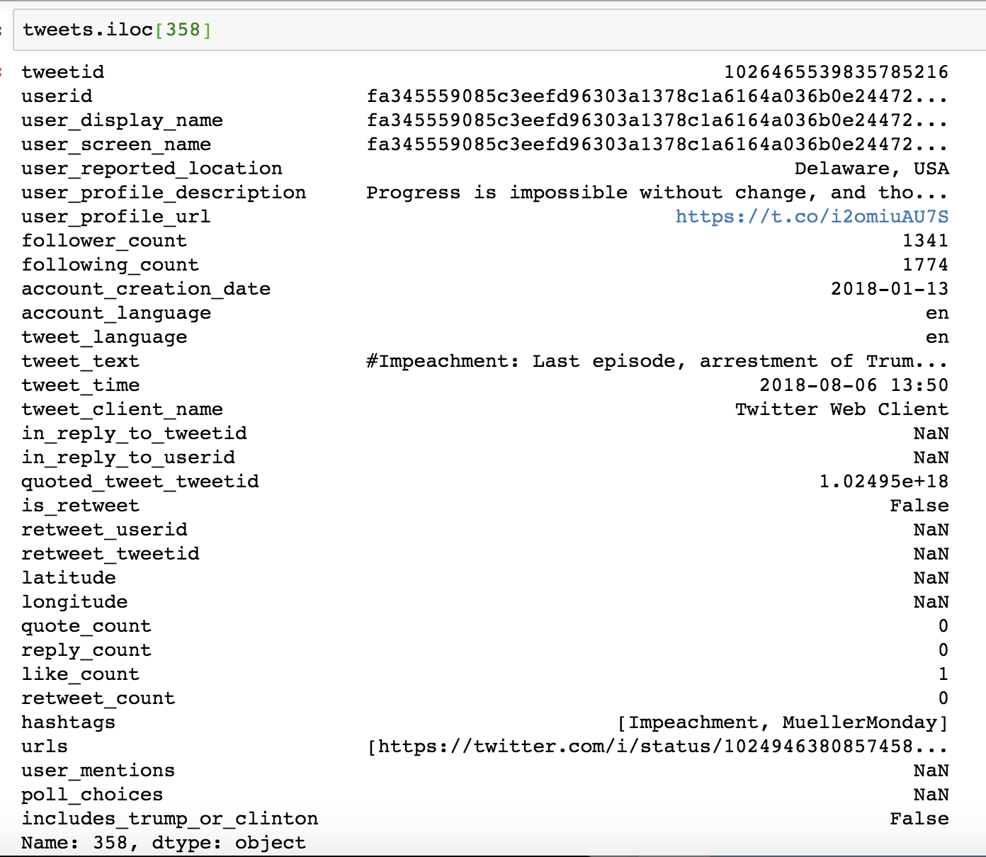
Figure 10-2: The values stored in the 359th row of our tweets’ DataFrame displayed using the .iloc[] method
The hashtags column, then, will allow us to identify tweets with hashtags that contain the strings trump or clinton. The tweet_time column contains a timestamp of when the tweet was sent. We’ll use the tweet_time column after we’ve filtered our data to calculate a monthly tally of Trump- and Clinton-related tweets.
To filter our data, we’ll repeat some of the same steps from our previous analysis of vaccination-related data. There, we created a new column and filled it with True or False by selecting another column and using the contains() function to see whether it contained the string vaccin. For this project, we’ll also create a True or False column, but instead of using the contains() function, we’ll be using a new pandas feature that’s much more powerful: lambda functions.
Lambdas
A lambda function is a small, nameless function we can apply to every value in a column. Instead of being confined to the functions that pandas developers have already written, like contains(), we can use custom lambdas to modify our data however we want.
Let’s take a look at the structure of a lambda function. Say we want to add 1 to a number and return the new number. A regular Python function for this might look like the following:
def add_one(x):

    return x + 1
Here we’ve used the def keyword to create a function and name it add_one(), defined x as the only parameter, and written our main line of code on an indented new line after a colon. Now let’s look at the lambda equivalent of the same function:
lambda x: x + 1
Unlike indented Python functions, lambdas are mostly written as compact one-liners and used inside of an apply() function. Instead of using def to write and name a new function, we’re using the word lambda followed by the parameter x (note that we don’t need to use the parentheses). Then we specify what we want to do to x—in this case, add 1. Notice that there’s no name for this function, which is why some people call lambdas anonymous functions.
To apply this lambda function to a column, we pass the function itself as an argument, as shown in Listing 10-1.
dataframe["column_name"].apply(lambda x: x + 1)
Listing 10-1: Passing a lambda function to apply()
In this example, we select the column with the name column_name from a hypothetical data frame called dataframe and apply the lambda x + 1 to it. (Note that for this to work, the values in column_name would need to be numbers, not strings.) This line of code would return a series of results that we’d get from adding 1 to the value of each row in the column_name column. In other words, it would display each value in the column_name column with 1 added to it.
In cases where you need to apply more-complex operations to a column, you can also pass traditional Python functions to apply(). For example, if we wanted to rewrite Listing 10-1 using the add_one() function we defined earlier, we’d simply pass the name into the apply() function, like so:
dataframe["column_name"].apply(add_one)
Lambdas can be a very helpful and efficient way for us to modify entire columns. They are ideal for one-off tasks, since they are unnamed (anonymous) and are easy and quick to write.
All right, enough about lambdas! Let’s get back to our analysis.
Filtering the Data Set
We want a data frame that contains only tweets relating to the 2016 presidential candidates. As mentioned before, we’re going to use a simple heuristic for this: include only tweets whose hashtags include the strings trump, clinton, or both. While this may not catch every tweet about Donald Trump or Hillary Clinton, it’s a clear-cut and easily understandable way to look at the activities of these misinformation agents.
First, we need to create a column that contains the Boolean values True or False, indicating whether a given tweet contains the string trump or clinton. We can use the code in Listing 10-2 to do this.
tweets["includes_trump_or_clinton"] = tweets["hashtags"].apply(lambda x: "clinton" in str(x).lower() or "trump" in str(x).lower())
Listing 10-2: Creating a new True or False column from our tweets data set
This code is pretty dense, so let’s break it down into parts. On the left side of the equal sign, we create a new column, includes_trump_or_clinton, that will store the results of our lambda function. Then, on the right side, we select the hashtags column and apply the following lambda function:
lambda x: "trump" in str(x).lower() or "clinton" in str(x).lower()
The first thing we do in the lambda function is check whether the string “trump” is within the longer string of hashtags using the line "trump" in str(x).lower(). This line takes the value passed in the hashtags column, x, uses the str() function to turn x into a string, uses the lower() function to make every letter in the string lowercase, and finally checks whether the string trump is in that lowercase string. If it is, then the function will return True; if it isn’t, it will return False. Using the str() function is a great way for us to turn any value we have to work with, even empty lists and NaN values, into strings that we can query; without str(), null values could cause errors in our code. It also lets us skip the step of filtering out null values, as we did in our analysis in Chapter 9.
On the other side of the or in our lambda function, we use the same code but for clinton. Thus, if the hashtag contains either the string trump or clinton (ignoring case), then the row will be filled with True; otherwise, it will be filled with False.
Once we have our True or False column, we need to filter our tweets down to only those with True values in includes_trump_or_clinton. We can do that with the code in Listing 10-3.
tweets_subset = tweets[tweets["includes_trump_or_clinton"] == True]
Listing 10-3: Filtering the tweets down to only those that include trump or clinton
This creates a new variable called tweets_subset that’ll store the reduced data frame containing only tweets that used Trump- or Clinton-related hashtags. Then we use the brackets to select the subset of tweets based on a condition—in this case, whether the value tweets["includes_trump_or_clinton"] is True.
Through these lines of code, we have now narrowed down our data set to the body of tweets that we’re interested in observing. We can use the code len(tweets_subset) in a separate cell to find out the number of rows in our tweets_subset, which should be 15,264. Now it’s time to see how the number of tweets containing Trump- or Clinton-related hashtags has changed over time.
Formatting the Data as datetimes
With our data set filtered, we want to count the number of tweets containing Trump- or Clinton-related hashtags within a certain time period—a count that is often referred to as a time series. To accomplish this, we’ll format the data columns as timestamps and use pandas functions to create tallies based on these timestamps.
As we saw during our adventures with Google Sheets in Chapter 6, it’s important that we specify to our code the kind of data we’re dealing with. Although Sheets and pandas can autodetect data types like integers, floats, and strings, they can make mistakes, so it’s better to be specific rather than leave it to chance. One way of doing that is by selecting the column that contains the timestamps for each tweet and telling Python to interpret them as a datetime data type.
First, though, we need to find out how pandas is currently interpreting our data columns. To do this, we’ll use the dtypes attribute, which, as you saw in Chapter 8, allows us to look at some characteristic of our data (in this case, the data types each column contains):
tweets_subset.dtypes
If we run this line in a cell, our Jupyter notebook should display a list of the columns in our data frame alongside their data type:
tweetid                       int64
userid                       object
user_display_name            object
user_screen_name             object
user_reported_location       object
user_profile_description     object
user_profile_url             object
follower_count                int64
following_count               int64
account_creation_date        object
account_language             object
tweet_language               object
tweet_text                   object
tweet_time                   object
tweet_client_name            object
in_reply_to_tweetid         float64
in_reply_to_userid           object
quoted_tweet_tweetid        float64
is_retweet                     bool
retweet_userid               object
retweet_tweetid             float64
latitude                    float6
longitude                   float64
quote_count                 float64
reply_count                 float64
like_count                  float64
retweet_count               float64
hashtags                     object
urls                         object
user_mentions                object
poll_choices                 object

dtype: object
As you can see here, there are two columns that contain time-related data: account_creation_date and tweet_time. We’re interested in understanding the tweets, not the accounts, so we’ll focus on tweet_time. Currently, pandas interprets the tweet_time column as an object data type, which in pandas most commonly means a string. But pandas has a data type specifically made for timestamps: datetime64[ns].
To format this data as datetime64[ns], we can use the pandas function astype(), which will replace the tweet_time column with a data column that contains the same data but interpreted as a datetime object. Listing 10-4 shows us how.
tweets_subset["tweet_time"] = tweets_subset["tweet_time"].astype("datetime64[ns]")
Listing 10-4: Formatting the data type of the tweet_time column using the asytype() function
As before, we select the “tweet_time” column by putting it in square brackets, and then we replace it by applying the .astype() function to it. In other words, this converts the selected column (tweet_time) into the data type we specify inside the parentheses ("datetime64[ns]").
To check whether our conversion worked, we can simply run dtypes on the tweets_subset variable again in a separate cell:
tweets_subset.dtypes
Below the cell containing this code, we should now see that the tweet_time column contains datetime64[ns] values.
--snip--

account_language                    object
tweet_language                      object
tweet_text                          object
tweet_time                  datetime64[ns]
tweet_client_name                   object
in_reply_to_tweetid                float64
in_reply_to_userid                  object
--snip--
Now that the tweet_time data is in the right data type, we can use it to start tallying up the values in includes_trump_or_clinton.
Resampling the Data
Remember that we’re hoping to find a count of the number of tweets containing Trump- or Clinton-related hashtags per time period. To do this, we’ll use a process called resampling, in which we aggregate data over specific time intervals; here, this could mean counting the number of tweets per day, per week, or per month. In our analysis, we’ll use a monthly tally, though if we wanted a more granular analysis, we might resample by week or even day.
The first step in resampling our data is to set tweet_time as an index (remember an index acts like a row label). This will allow us to select and locate entries based on their tweet_time value, and later apply different kinds of mathematical operations to it.
To set the tweet_time column as an index, we can use the set_index() function. We apply set_index() to tweet_time by passing tweet_time as its argument. The set_index() function will return a newly indexed data frame, which we’ll store in a variable called tweets_over_time (Listing 10-5).
tweets_over_time = tweets_subset.set_index(“tweet_time”)
Listing 10-5: Setting a new index and storing the resulting data frame
To see what a newly indexed data frame looks like, run the tweets_over_time.head() function, which should return something like Figure 10-3.
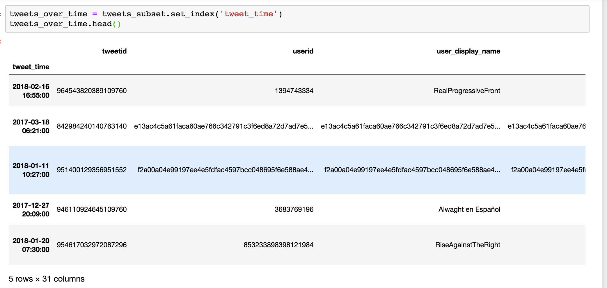
Figure 10-3: A data frame that has taken on the tweet_time column as an index
There’s a subtle but important visual change here: the values in the tweet_time column have replaced the integer-based index numbers on the left side of our data and are now displayed in bold. This means that we’ve replaced the number-based indexes with timestamps in the tweet_time column.
With our new index, we can group and aggregate our data over time using the resample() function, as in Listing 10-6.
tweet_tally = tweets_over_time.resample("M").count()
Listing 10-6: Grouping and aggregating data in a data frame using resample()
We can specify the frequency at which we want to aggregate our data over time—every day, every week, or every month—inside the resample() function’s parentheses. In this case, because we’re interested in how these tweets may have been used to influence the 2016 US presidential election, we want a monthly tally, so we pass in the string “M” (short for month). Last but not least, we need to specify how we want to aggregate our data over time. Since we want a monthly count of tweets, we’ll use the count() function.
Once we run this cell, we can run tweet_tally.head() in a new cell to look at our data. We should see a data frame containing a count of all the values in each column per month, as shown in Figure 10-4.
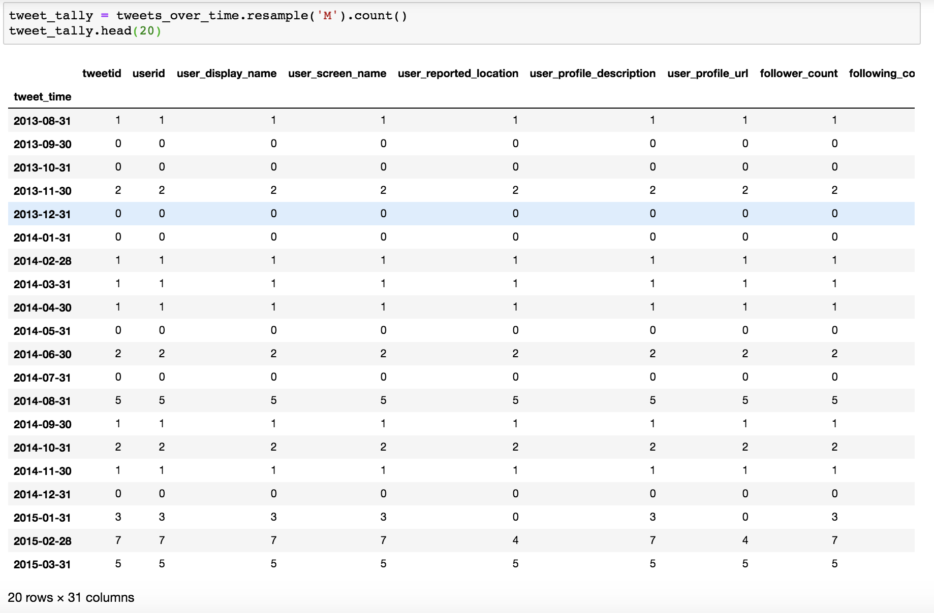
Figure 10-4: A resampled data frame containing the monthly counts for each column value. Note the variance in counts for the data in the row indexed as 2015-01-31.
As you can see, pandas has counted the number of values contained in every column for each month and stored that result as the new column value. Every row now represents one month, beginning with the date in tweet_time.
That result is not ideal. We now have a lot of values strewn across some 30 columns, and in addition to that, the counts in each column for a given month can vary, too. Take the row labeled 2015-01-31 in Figure 10-4, for instance. For that month, we counted zero values in the user_profile_url column even though the count in the tweet_id column is 3. That means that the Iranian agents posted three tweets with hashtags containing the strings trump or clinton during that month, but none of them contained a user profile URL.
Based on this observation, we should be careful about what we rely on to best determine the total number of tweets per month—we should be careful about which values we count. If we counted the number of values in the user_profile_url column, we would only catch the tweets that featured user profile URLs; we wouldn’t be catching the tweets that didn’t feature those URLs, and we would be undercounting the number of overall tweets that are in our data frame.
So before we even resample our data set, we should look at a data column that contains a value for every single row and count those values. This is a critically important step: there are values that may seem like they occur in every row when we render the data using the head() or tail() function, but we can’t be sure of that simply by looking at one relatively small part of a massive data set. It helps to think about what column most reliably represents a distinct entity that cannot be omitted in the data collection (for example, a tweet may not always contain a tag, but it must have a unique identifier or ID). In the data set that is stored in the tweets_over_time variable back in Listing 10-5, there is a value in every row of the tweetid column.
Because we need only the total number of tweets per month, we can use only the tweetid column, which we’ll store in the variable monthly_tweet_count as follows:
monthly_tweet_count = tweet_tally["tweetid"]
Now, if we inspect our monthly_tweet_count using the head() function, we get a much cleaner monthly tally of our data frame:
tweet_time
2013-08-31    1
2013-09-30    0
2013-10-31    0
2013-11-30    2
2013-12-31    0

Freq: M, Name: tweetid, dtype: int64
Our code has now created a data frame that allows us to better understand our data over time, but this row-by-row preview is still limited. We want to see the major trends across the entire data set.
Plotting the Data
To get a fuller picture of our data, we’ll use matplotlib, the library that we installed and imported earlier in this chapter. The matplotlib library allows us to plot and visualize pandas data frames—perfect for this project, as time series are often much clearer when visualized.
At the beginning of this project, we imported the matplotlib library’s pyplot functions as plt. To access these functions, we type plt followed by the function we want to use, as follows:
plt.plot(monthly_tweet_count)
In this case, we use the plot() function, with our data frame monthly_tweet_count as its argument, to plot the dates of our data frame on the x-axis and the number of tweets per month on the y-axis, as shown in Figure 10-5.
Note There are many ways to customize plots in matplotlib; to learn more about them, go to https://matplotlib.org/.
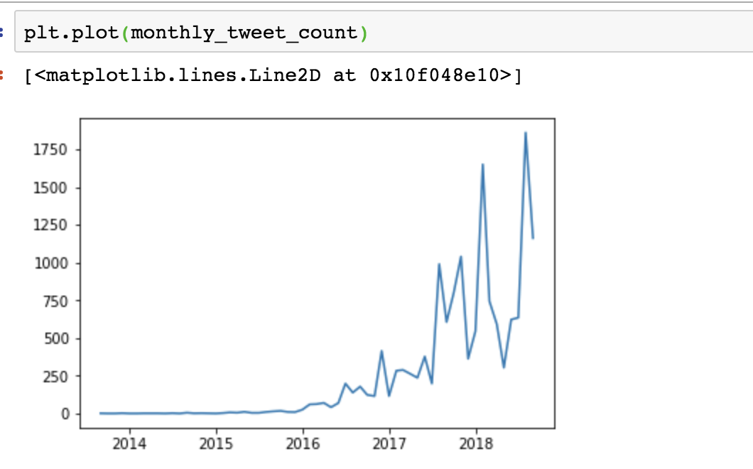
Figure 10-5: A chart created by matplotlib inside Jupyter Notebook
Ta-da! Now we have a graph that shows the number of tweets that used Trump- or Clinton-related hashtags. As we might’ve expected, they increased drastically toward the end of 2016, showing us that these false agents became very active in the lead-up to, and aftermath of, the 2016 US presidential election—though there seems to be a lot of variability in their activities several months after the election took place. While we won’t be able to do all the research necessary to explain this activity, researchers at the Digital Forensics Research Lab have published a deeper analysis of the Iranian accounts at https://web.archive.org/web/20190504181644/.
Summary
This project has demonstrated the power of doing data analysis in Python. With a few lines of code, we were able to open a massive data set, filter it based on its contents, summarize it into monthly counts, and visualize it for better understanding. Along the way, you learned about lambda functions and resampling data based on datetime objects.
This chapter concludes the practical exercises for the book. In the next, and final, chapter, we’ll discuss how you can take these introductory lessons further on your own to become an active and self-sufficient Python learner.